Start Simulation Async

This example sets up and solves a simulation of particles interacting with a rotating L-shape tube wall using an async call.

Perform imports and create a project

Perform the required imports and create an empty project.

import os
import tempfile
import time

import ansys.rocky.core as pyrocky
from ansys.rocky.core import examples

awp_roots = sorted(
    [k for k in os.environ.keys() if k.startswith("AWP_ROOT")], reverse=True
)
last_rocky_version = int(awp_roots[0].partition("AWP_ROOT")[2])
if last_rocky_version >= 251:
    # `non_blocking` simulation only available on Rocky 25R1 and onwards.

    # Create a temp directory to save the project.
    project_dir = tempfile.mkdtemp(prefix="pyrocky_")

    # Launch Rocky and open a project.
    rocky = pyrocky.launch_rocky()
    project = rocky.api.CreateProject()
    project.SaveProject(os.path.join(project_dir, "rocky-testing.rocky"))

    ###############################################################################
    # Configure the study
    # ~~~~~~~~~~~~~~~~~~~
    study = project.GetStudy()

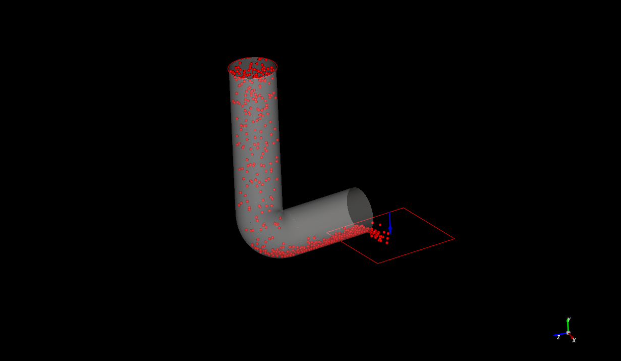
    # Download the STL file that was imported into Rocky to represent a wall.
    file_name = "Lshape_tube.stl"
    file_path = examples.download_file(project_dir, file_name, "pyrocky/geometries")
    wall = study.ImportWall(file_path)[0]

    # Create a particle with the default shape (sphere) and size distribution (single
    # distribution with a sieve size of 0.1 m).
    particle = study.CreateParticle()

    # Create a circular surface to used as the inlet.
    circular_surface = study.CreateCircularSurface()
    circular_surface.SetMaxRadius(0.8, unit="m")

    # Create a rectangular surface to use as the outlet.
    rectangular_surface = study.CreateRectangularSurface()
    rectangular_surface.SetLength(3, unit="m")
    rectangular_surface.SetWidth(3, unit="m")
    rectangular_surface.SetCenter((5, -7.5, 0), unit="m")

    # Set the inlet and outlet.
    particle_inlet = study.CreateParticleInlet(circular_surface, particle)
    input_property_list = particle_inlet.GetInputPropertiesList()
    input_property_list[0].SetMassFlowRate(1000)
    outlet = study.CreateOutlet(rectangular_surface)

    # Set the motion rotation over the Y axis and apply it on the wall and the
    # rectangular surface used as the outlet.
    motion_frame_source = study.GetMotionFrameSource()
    motion_frame = motion_frame_source.NewFrame()
    motion_frame.AddRotationMotion(angular_velocity=((0.0, 0.5, 0.0), "rad/s"))
    motion_frame.ApplyTo(rectangular_surface)
    motion_frame.ApplyTo(wall)

    # The domain settings define the domain limits where the particles are enabled to be
    # computed in the simulation.
    domain = study.GetDomainSettings()
    domain.DisableUseBoundaryLimits()
    domain.SetCoordinateLimitsMaxValues((10, 1, 10), unit="m")

    ###############################################################################
    # Set up the solver and run the simulation
    # ~~~~~~~~~~~~~~~~~~~~~~~~~~~~~~~~~~~~~~~~

    solver = study.GetSolver()
    simulation_duration = 5
    solver.SetSimulationDuration(simulation_duration, unit="s")
    # `non_blocking` only available on Rocky 25R1 and onwards.
    study.StartSimulation(non_blocking=True)

    ###############################################################################
    # Postprocess
    # ~~~~~~~~~~~
    # Obtain the in and out mass flows of the particles while the simulation is
    # running.
    particles = study.GetParticles()

    while study.IsSimulating():
        # When running an asynchronous simulation, the call to RefreshResults is required
        # to ensure that the results are updated.
        study.RefreshResults()

        times, mass_flow_in = particles.GetNumpyCurve(
            "Particles Mass Flow In", unit="t/h"
        )
        times, mass_flow_out = particles.GetNumpyCurve(
            "Particles Mass Flow Out", unit="t/h"
        )

        print(f"Simulation Progress: {study.GetProgress():.2f} %")
        print(f"\tCurrent mass_flow_in: {mass_flow_in[-1]:.2f} t/h")
        print(f"\tCurrent mass_flow_out: {mass_flow_out[-1]:.2f} t/h")

        time.sleep(2)

    print("Simulation Complete!")

    times, mass_flow_in = particles.GetNumpyCurve("Particles Mass Flow In", unit="t/h")
    times, mass_flow_out = particles.GetNumpyCurve("Particles Mass Flow Out", unit="t/h")

    # Obtain the maximum and minimum velocities of the particles at each time step.
    import numpy as np

    simulation_times = study.GetTimeSet()
    velocity_gf = particles.GetGridFunction("Velocity : Translational : Absolute")
    velocity_max = np.array(
        [
            velocity_gf.GetMax(unit="m/s", time_step=i)
            for i in range(len(simulation_times))
        ]
    )
    velocity_min = np.array(
        [
            velocity_gf.GetMin(unit="m/s", time_step=i)
            for i in range(len(simulation_times))
        ]
    )

    #################################################################################
    # Plot curves
    # +++++++++++

    import matplotlib.pyplot as plt

    fig, (ax1, ax2) = plt.subplots(2, 1)

    ax1.plot(times, mass_flow_in, "b", label="Mass Flow In")
    ax1.plot(times, mass_flow_out, "r", label="Mass Flow Out")
    ax1.set_xlabel("Time [s]")
    ax1.set_ylabel("Mass Flow [t/h]")
    ax1.legend(loc="upper left")

    ax2.plot(simulation_times, velocity_max, "b", label="Max Velocity")
    ax2.plot(simulation_times, velocity_min, "r", label="Min Velocity")
    ax2.set_xlabel("Time [s]")
    ax2.set_ylabel("Velocity [m/s]")
    ax2.legend(loc="upper left")

    plt.draw()

    rocky.close()